

一、简介
本项目是对论文《Stock Trading with Recurrent Reinforcement Learning (RRL)》的代码重现。
论文URL:http://cs229.stanford.edu/proj2006/Molina-StockTradingWithRecurrentReinforcementLearning.pdf
二、结论
先看结论吧:
这种方法的主要困难在于某些股票事件没有显示结构。从上面的第二个示例中可以看出,强化学习者无法预测股价的急剧下跌,并且像人类一样脆弱。如果与预测这种急剧下降的机制结合使用,可能会更有效。该模型还可以在其他方面作出修改,比如将成交量包含进来,作为预测涨跌的特征。
另外,可以尝试使用固定交易成本以及降低交易频率。例如,可以创建一个模型,该模型从长时间的数据中学习,但只能定期做出决策。这将反映一个散户交易者以固定交易成本参与较小数量交易的情况。因为对于散户而言,以固定的交易成本在每个期间进行交易都太昂贵了,所以具有定期交易策略的模型对于此类用户更为可行。
三、小知识
1.Sharp夏普比率的计算方法

四、代码
# -*- coding: utf-8 -*-
import time
import pickle
import numpy as np
import pandas as pd
from datetime import datetime as dt
import matplotlib.pyplot as plt


def main():

    fname = "../data/USDJPY30.csv"
    init_t = 6000

    T = 1000
    M = 200
    mu = 10000
    sigma = 0.04
    rho = 1.0
    n_epoch = 10000

    # RRL agent with initial weight.
    ini_rrl = TradingRRL(T, M, init_t, mu, sigma, rho, n_epoch)
    ini_rrl.load_csv(fname)
    ini_rrl.set_t_p_r()
    ini_rrl.calc_dSdw()
    # RRL agent for training
    rrl = TradingRRL(T, M, init_t,  mu, sigma, rho, n_epoch)
    rrl.all_t = ini_rrl.all_t
    rrl.all_p = ini_rrl.all_p
    rrl.set_t_p_r()
    rrl.fit()

    # Plot results.
    # Training for initial term T.
    plt.plot(range(len(rrl.epoch_S)),rrl.epoch_S)
    plt.title("Sharp's ratio optimization")
    plt.xlabel("Epoch times")
    plt.ylabel("Sharp's ratio")
    plt.grid(True)
    plt.savefig("sharp's ratio optimization.png", dpi=300)
    plt.close

    fig, ax = plt.subplots(nrows=3, figsize=(15, 10))
    t = np.linspace(1, rrl.T, rrl.T)[::-1]
    ax[0].plot(t, rrl.p[:rrl.T])
    ax[0].set_xlabel("time")
    ax[0].set_ylabel("USDJPY")
    ax[0].grid(True)

    ax[1].plot(t, ini_rrl.F[:rrl.T], color="blue", label="With initial weights")
    ax[1].plot(t, rrl.F[:rrl.T], color="red", label="With optimized weights")
    ax[1].set_xlabel("time")
    ax[1].set_ylabel("F")
    ax[1].legend(loc="upper left")
    ax[1].grid(True)

    ax[2].plot(t, ini_rrl.sumR, color="blue", label="With initial weights")
    ax[2].plot(t, rrl.sumR, color="red", label="With optimized weights")
    ax[2].set_xlabel("time")
    ax[2].set_ylabel("Sum of reward[yen]")
    ax[2].legend(loc="upper left")
    ax[2].grid(True)
    plt.savefig("rrl_train.png", dpi=300)
    fig.clear()


    # Prediction for next term T with optimized weight.
    # RRL agent with initial weight.
    ini_rrl_f = TradingRRL(T, M, init_t-T, mu, sigma, rho, n_epoch)
    ini_rrl_f.all_t = ini_rrl.all_t
    ini_rrl_f.all_p = ini_rrl.all_p
    ini_rrl_f.set_t_p_r()
    ini_rrl_f.calc_dSdw()
    # RRL agent with optimized weight.
    rrl_f = TradingRRL(T, M, init_t-T, mu, sigma, rho, n_epoch)
    rrl_f.all_t = ini_rrl.all_t
    rrl_f.all_p = ini_rrl.all_p
    rrl_f.set_t_p_r()
    rrl_f.w = rrl.w
    rrl_f.calc_dSdw()

    fig, ax = plt.subplots(nrows=3, figsize=(15, 10))
    t_f = np.linspace(rrl.T+1, rrl.T+rrl.T, rrl.T)[::-1]
    ax[0].plot(t_f, rrl_f.p[:rrl_f.T])
    ax[0].set_xlabel("time")
    ax[0].set_ylabel("USDJPY")
    ax[0].grid(True)

    ax[1].plot(t_f, ini_rrl_f.F[:rrl_f.T], color="blue", label="With initial weights")
    ax[1].plot(t_f, rrl_f.F[:rrl_f.T], color="red", label="With optimized weights")
    ax[1].set_xlabel("time")
    ax[1].set_ylabel("F")
    ax[1].legend(loc="lower right")
    ax[1].grid(True)

    ax[2].plot(t_f, ini_rrl_f.sumR, color="blue", label="With initial weights")
    ax[2].plot(t_f, rrl_f.sumR, color="red", label="With optimized weights")
    ax[2].set_xlabel("time")
    ax[2].set_ylabel("Sum of reward[yen]")
    ax[2].legend(loc="lower right")
    ax[2].grid(True)
    plt.savefig("rrl_prediction.png", dpi=300)
    fig.clear()

class TradingRRL(object):
    def __init__(self, T=1000, M=200, init_t=10000, mu=10000, sigma=0.04, rho=1.0, n_epoch=10000):
        self.T = T
        self.M = M
        self.init_t = init_t
        self.mu = mu
        self.sigma = sigma
        self.rho = rho
        self.all_t = None
        self.all_p = None
        self.t = None
        self.p = None
        self.r = None
        self.x = np.zeros([T, M+2])
        self.F = np.zeros(T+1)
        self.R = np.zeros(T)
        self.w = np.ones(M+2)
        self.w_opt = np.ones(M+2)
        self.epoch_S = np.empty(0)
        self.n_epoch = n_epoch
        self.progress_period = 100
        self.q_threshold = 0.7

    def load_csv(self, fname):
        tmp = pd.read_csv(fname, header=None)
        tmp_tstr = tmp[0] +" " + tmp[1]
        tmp_t = [dt.strptime(tmp_tstr[i], '%Y.%m.%d %H:%M') for i in range(len(tmp_tstr))]
        tmp_p = list(tmp[5])
        self.all_t = np.array(tmp_t[::-1])
        self.all_p = np.array(tmp_p[::-1])

    def quant(self, f):
        fc = f.copy()
        fc[np.where(np.abs(fc) < self.q_threshold)] = 0
        return np.sign(fc)

    def set_t_p_r(self):
        self.t = self.all_t[self.init_t:self.init_t+self.T+self.M+1]
        self.p = self.all_p[self.init_t:self.init_t+self.T+self.M+1]
        self.r = -np.diff(self.p)

    def set_x_F(self):
        for i in range(self.T-1, -1 ,-1):
            self.x[i] = np.zeros(self.M+2)
            self.x[i][0] = 1.0
            self.x[i][self.M+2-1] = self.F[i+1]
            for j in range(1, self.M+2-1, 1):
                self.x[i][j] = self.r[i+j-1]
            self.F[i] = np.tanh(np.dot(self.w, self.x[i]))

    def calc_R(self):
        self.R = self.mu * (self.F[1:] * self.r[:self.T] - self.sigma * np.abs(-np.diff(self.F)))

    def calc_sumR(self):
        self.sumR  = np.cumsum(self.R[::-1])[::-1]
        self.sumR2  = np.cumsum((self.R**2)[::-1])[::-1]

    def calc_dSdw(self):
        self.set_x_F()
        self.calc_R()
        self.calc_sumR()
        self.A      =  self.sumR[0] / self.T
        self.B      =  self.sumR2[0] / self.T
        self.S      =  self.A / np.sqrt(self.B - self.A**2)
        self.dSdA   =  self.S * (1 + self.S**2) / self.A
        self.dSdB   = -self.S**3 / 2 / self.A**2
        self.dAdR   =  1.0 / self.T
        self.dBdR   =  2.0 / self.T * self.R
        self.dRdF   = -self.mu * self.sigma * np.sign(-np.diff(self.F))
        self.dRdFp  =  self.mu * self.r[:self.T] + self.mu * self.sigma * np.sign(-np.diff(self.F))
        self.dFdw   = np.zeros(self.M+2)
        self.dFpdw  = np.zeros(self.M+2)
        self.dSdw   = np.zeros(self.M+2)
        for i in range(self.T-1, -1 ,-1):
            if i != self.T-1:
                self.dFpdw = self.dFdw.copy()
            self.dFdw  = (1 - self.F[i]**2) * (self.x[i] + self.w[self.M+2-1] * self.dFpdw)
            self.dSdw += (self.dSdA * self.dAdR + self.dSdB * self.dBdR[i]) * (self.dRdF[i] * self.dFdw + self.dRdFp[i] * self.dFpdw)

    def update_w(self):
        self.w += self.rho * self.dSdw

    def fit(self):

        pre_epoch_times = len(self.epoch_S)

        self.calc_dSdw()
        print("Epoch loop start. Initial sharp's ratio is " + str(self.S) + ".")
        self.S_opt = self.S

        tic = time.clock()
        for e_index in range(self.n_epoch):
            self.calc_dSdw()
            if self.S > self.S_opt:
                self.S_opt = self.S
                self.w_opt = self.w.copy()
            self.epoch_S = np.append(self.epoch_S, self.S)
            self.update_w()
            if e_index % self.progress_period  == self.progress_period-1:
                toc = time.clock()
                print("Epoch: " + str(e_index + pre_epoch_times + 1) + "/" + str(self.n_epoch + pre_epoch_times) +". Shape's ratio: " + str(self.S) + ". Elapsed time: " + str(toc-tic) + " sec.")
        toc = time.clock()
        print("Epoch: " + str(e_index + pre_epoch_times + 1) + "/" + str(self.n_epoch + pre_epoch_times) +". Shape's ratio: " + str(self.S) + ". Elapsed time: " + str(toc-tic) + " sec.")
        self.w = self.w_opt.copy()
        self.calc_dSdw()
        print("Epoch loop end. Optimized sharp's ratio is " + str(self.S_opt) + ".")

    def save_weight(self):
        pd.DataFrame(self.w).to_csv("w.csv", header=False, index=False)
        pd.DataFrame(self.epoch_S).to_csv("epoch_S.csv", header=False, index=False)

    def load_weight(self):
        tmp = pd.read_csv("w.csv", header=None)
        self.w = tmp.T.values[0]


def plot_hist(n_tick, R):
    rnge = max(R) - min(R)
    tick = rnge / n_tick
    tick_min = [min(R) - tick * 0.5 + i * tick for i in range(n_tick)]
    tick_max = [min(R) + tick * 0.5 + i * tick for i in range(n_tick)]
    tick_center = [min(R) + i * tick for i in range(n_tick)]
    tick_val = [0.0] * n_tick
    for i in range(n_tick ):
        tick_val[i] = len(set(np.where(tick_min[i] < np.array(R))[0].tolist()).intersection(np.where(np.array(R) <= tick_max[i])[0]))
    plt.bar(tick_center, tick_val, width=tick)
    plt.grid()
    plt.show()


if __name__ == "__main__":
    main()
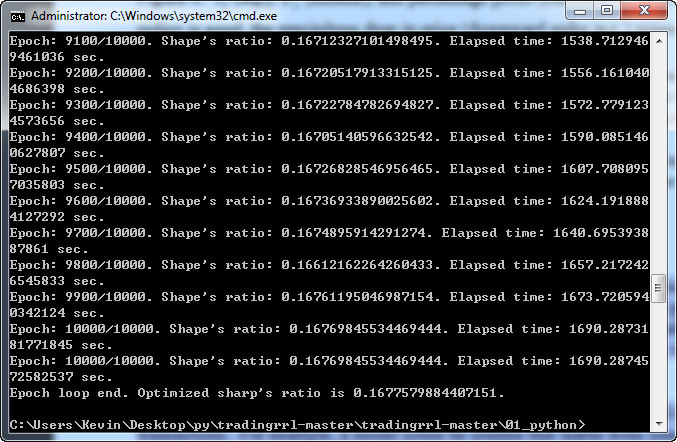
运行截图:
可参考:
https://zhuanlan.zhihu.com/p/36632686
代码地址:https://github.com/darden1/tradingrrl