蜗牛之路

一、结果
数据时间范围: 2025-06-06 09:31:00 至 2026-01-09 15:00:00
总分钟数: 35366

生成的基础因子列表：
['ret_1m', 'ret_5m', 'ret_15m', 'corr_vp', 'illiq', 'illiq_ma', 'up_vol', 'down_vol', 'imb', 'rv', 'rv_ratio', 'mom', 'overnight_ret', 'intraday_ret', 'reversal', 'upper_shadow', 'lower_shadow', 'pressure', 'vwap', 'vwap_dev', 'direction', 'buy_vol', 'sell_vol', 'net_vol', 'vol_ratio']

=== 开始遗传规划因子挖掘 ===
各因子缺失比例：
ret_1m 0.000028
ret_5m 0.000141
ret_15m 0.000424
corr_vp 0.000820
illiq_ma 0.000848
imb 0.000537
rv_ratio 0.004213
mom 0.000848
reversal 0.000679
pressure 0.000537
vwap_dev 0.000820
vol_ratio 0.000820
dtype: float64

实际用于遗传规划的因子列 (12个): ['ret_1m', 'ret_5m', 'ret_15m', 'corr_vp', 'illiq_ma', 'imb', 'rv_ratio', 'mom', 'reversal', 'pressure', 'vwap_dev', 'vol_ratio']
遗传规划可用数据行数: 35183（总行数: 35366）

=== 目标收益诊断 ===
count 35183.000000
mean 0.000032
std 0.003392
min -0.022635
25% -0.001720
50% 0.000000
75% 0.001729
max 0.027119
Name: future_ret_30, dtype: float64
标准差: 0.0033915940902883566
唯一值个数: 3480
因子 ret_1m 与目标收益的 Rank IC: -0.080238
因子 ret_5m 与目标收益的 Rank IC: -0.042970
因子 ret_15m 与目标收益的 Rank IC: -0.013608

[调试] 个体 #1 因子值统计：
均值: 0.211265, 标准差: 0.243985
最小值: 0.000000, 最大值: 0.968815
唯一值数量: 29917 (总样本: 35183)
表达式: maximum(safe_sqrt(add(imb, ret_15m)), absolute(multiply(ret_5m, imb)))

[调试] 个体 #2 因子值统计：
均值: 0.357712, 标准差: 0.191625
最小值: -0.424701, 最大值: 0.925192
唯一值数量: 32303 (总样本: 35183)
表达式: maximum(reversal, imb)

[调试] 个体 #3 因子值统计：
均值: -482.225127, 标准差: 3795.481609
最小值: -31941.113993, 最大值: 30077.296492
唯一值数量: 35183 (总样本: 35183)
表达式: add(safe_div(safe_div(imb, mom), safe_sqrt(mom)), absolute(subtract(ret_15m, rv_ratio)))
gen nevals avg max
0 100 0 0
1 76 0 0
2 72 0 0
3 66 0 0
4 65 0 0
5 71 0 0
6 73 0 0
7 76 0 0
8 71 0 0
9 78 0 0
10 74 0 0
11 66 0 0
12 65 0 0
13 70 0 0
14 68 0 0
15 76 0 0
16 69 0 0
17 71 0 0
18 75 0 0
19 76 0 0
20 68 0 0

最佳因子表达式： maximum(safe_sqrt(add(imb, ret_15m)), absolute(multiply(ret_5m, imb)))
遗传规划因子已保存至 'gp_factor' 列。

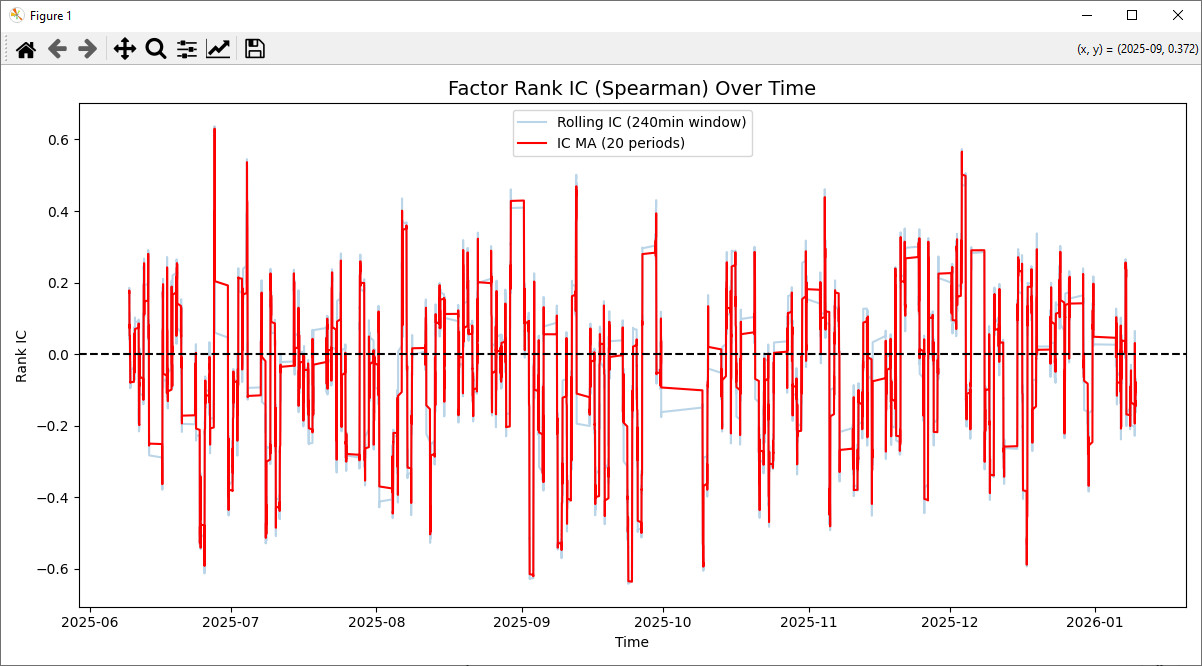
=== 单资产因子 IC 分析 ===
有效分析行数: 35336
Rank IC 均值: -0.045576
Rank IC 标准差: 0.203547
IR (Information Ratio): -0.2239
IC 正比例: 42.87%

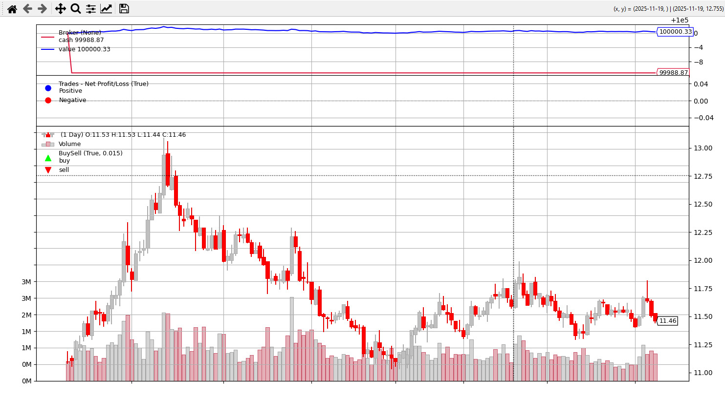
=== Backtrader策略回测 ===
初始资金: 100000.00
最终资金: 100000.33
年化收益率: 0.00%
夏普比率: -8822.30
最大回撤: 0.00%
PS I:\量化交易\yinzi>

二、代码

# ==================== 0. 环境准备 ====================
import pandas as pd
import numpy as np
import random
from datetime import datetime, time
import warnings
warnings.filterwarnings('ignore')

# 遗传规划库
from deap import base, creator, tools, gp, algorithms

# 因子分析库
import alphalens as al

# 回测库
import backtrader as bt
import backtrader.analyzers as btanalyzers

# ==================== 1. 数据加载与预处理 ====================
# 假设数据已保存为 'data.csv'，格式与你给出的样例一致
df_raw = pd.read_csv('data.csv', encoding='gbk')

# 合并日期和时间列，生成精确到分钟的datetime索引
df_raw['datetime'] = pd.to_datetime(df_raw['日期'].astype(str) + ' ' + df_raw['时间'])
df_raw.drop(['日期', '时间'], axis=1, inplace=True)
df_raw.set_index('datetime', inplace=True)
df_raw.sort_index(inplace=True)

# 提取股票代码（假设只有一只股票，但保留结构以支持多只）
stock_code = df_raw['股票代码'].iloc[0]

# 仅保留需要的OHLCV列
df = df_raw[['open', 'high', 'low', 'close', 'volume', '成交额']].copy()
df.rename(columns={'成交额': 'amount'}, inplace=True)

# 过滤集合竞价时段 (9:15-9:25) —— 根据样例，数据从9:31开始，无需过滤，但保留逻辑
def is_trading_time(ts):
    t = ts.time()
    morning = (time(9,30) <= t <= time(11,30))
    afternoon = (time(13,0) <= t <= time(15,0))
    return morning or afternoon

df = df[df.index.map(is_trading_time)]

print(f"数据时间范围: {df.index[0]} 至 {df.index[-1]}")
print(f"总分钟数: {len(df)}")

# ==================== 2. 基础因子计算引擎（1分钟专用） ====================
class OneMinFactorGenerator:
    def __init__(self, df_min):
        self.df = df_min.copy()
        self.df.sort_index(inplace=True)
        
    def factor_returns(self):
        self.df['ret_1m'] = self.df['close'].pct_change()
        self.df['ret_5m'] = self.df['close'].pct_change(5)
        self.df['ret_15m'] = self.df['close'].pct_change(15)
        return self.df[['ret_1m', 'ret_5m', 'ret_15m']]
    
    def factor_volume_price_corr(self, window=30):
        self.df['corr_vp'] = self.df['volume'].rolling(window).corr(self.df['close'])
        return self.df[['corr_vp']]
    
    def factor_illiquidity(self, window=30):
        self.df['illiq'] = np.abs(self.df['ret_1m']) / (self.df['amount'] / 1e6)
        self.df['illiq_ma'] = self.df['illiq'].rolling(window).mean()
        return self.df[['illiq_ma']]
    
    def factor_order_imbalance(self, window=20):
        self.df['up_vol'] = np.where(self.df['close'] > self.df['open'], self.df['volume'], 0)
        self.df['down_vol'] = np.where(self.df['close'] < self.df['open'], self.df['volume'], 0)
        self.df['imb'] = (self.df['up_vol'].rolling(window).sum() - 
                          self.df['down_vol'].rolling(window).sum()) / \
                         (self.df['volume'].rolling(window).sum() + 1e-9)
        return self.df[['imb']]
    
    def factor_high_freq_volatility(self, window=30):
        self.df['rv'] = np.sqrt((self.df['ret_1m']**2).rolling(window).sum() * 240)
        self.df['rv_ratio'] = self.df['rv'] / self.df['rv'].rolling(120).mean()
        return self.df[['rv_ratio']]
    
    def factor_intraday_momentum(self, short=10, long=30):
        self.df['mom'] = self.df['close'].pct_change(short) - self.df['close'].pct_change(long)
        return self.df[['mom']]
    
    def factor_intraday_reversal(self, window=20):
        self.df['overnight_ret'] = self.df['open'] / self.df['close'].shift(1) - 1
        self.df['intraday_ret'] = self.df['close'] / self.df['open'] - 1
        self.df['reversal'] = -self.df['overnight_ret'].rolling(window).corr(self.df['intraday_ret'])
        return self.df[['reversal']]
    
    def factor_order_book_pressure(self, window=20):
        self.df['upper_shadow'] = (self.df['high'] - np.maximum(self.df['open'], self.df['close'])) / self.df['close']
        self.df['lower_shadow'] = (np.minimum(self.df['open'], self.df['close']) - self.df['low']) / self.df['close']
        self.df['pressure'] = (self.df['upper_shadow'].rolling(window).mean() - 
                                self.df['lower_shadow'].rolling(window).mean())
        return self.df[['pressure']]
    
    def factor_vwap_deviation(self, window=30):
        self.df['vwap'] = (self.df['amount'] / self.df['volume']).rolling(window).mean()
        self.df['vwap_dev'] = self.df['close'] / self.df['vwap'] - 1
        return self.df[['vwap_dev']]
    
    def factor_tick_rule_volume(self, window=30):
        self.df['direction'] = np.sign(self.df['close'].diff())
        self.df['buy_vol'] = np.where(self.df['direction'] > 0, self.df['volume'], 0)
        self.df['sell_vol'] = np.where(self.df['direction'] < 0, self.df['volume'], 0)
        self.df['net_vol'] = (self.df['buy_vol'].rolling(window).sum() - 
                              self.df['sell_vol'].rolling(window).sum())
        self.df['vol_ratio'] = self.df['net_vol'] / (self.df['volume'].rolling(window).sum() + 1e-9)
        return self.df[['vol_ratio']]
    
    def generate_all_factors(self):
        self.factor_returns()
        self.factor_volume_price_corr()
        self.factor_illiquidity()
        self.factor_order_imbalance()
        self.factor_high_freq_volatility()
        self.factor_intraday_momentum()
        self.factor_intraday_reversal()
        self.factor_order_book_pressure()
        self.factor_vwap_deviation()
        self.factor_tick_rule_volume()
        return self.df

# 生成基础因子
gen = OneMinFactorGenerator(df)
factor_df = gen.generate_all_factors()
print("\n生成的基础因子列表：")
print(])

# ==================== 3. 因子预处理与涨跌停屏蔽 ====================
def handle_limit_up_down(df, limit_threshold=0.095):
    df['limit_up'] = (df['close'].pct_change() > limit_threshold)
    df['limit_down'] = (df['close'].pct_change() < -limit_threshold)
    # 触及涨跌停后因子值置NaN
    factor_cols = ]
    for col in factor_cols:
        df.loc[df['limit_up'] | df['limit_down'], col] = np.nan
    return df

factor_df = handle_limit_up_down(factor_df)

# ==================== 4. 遗传规划因子挖掘（DEAP） ====================
print("\n=== 开始遗传规划因子挖掘 ===")

# ---------- 4.1 筛选有效因子列 ----------
factor_columns = ['ret_1m', 'ret_5m', 'ret_15m', 'corr_vp', 'illiq_ma',
                  'imb', 'rv_ratio', 'mom', 'reversal', 'pressure', 'vwap_dev', 'vol_ratio']

missing_ratio = factor_df[factor_columns].isnull().mean()
print("各因子缺失比例：")
print(missing_ratio)

valid_factor_cols = missing_ratio[missing_ratio <= 0.8].index.tolist()
print(f"\n实际用于遗传规划的因子列 ({len(valid_factor_cols)}个): {valid_factor_cols}")

# ---------- 4.2 构建遗传规划数据集 ----------
factor_df['future_ret_30'] = factor_df['close'].pct_change(30).shift(-30)

gp_data = factor_df[valid_factor_cols + ['future_ret_30']].dropna()
print(f"遗传规划可用数据行数: {len(gp_data)}（总行数: {len(factor_df)}）")

# 诊断目标收益质量
print("\n=== 目标收益诊断 ===")
print(gp_data['future_ret_30'].describe())
print("标准差:", gp_data['future_ret_30'].std())
print("唯一值个数:", gp_data['future_ret_30'].nunique())
for col in valid_factor_cols[:3]:
    ic = gp_data[col].corr(gp_data['future_ret_30'], method='spearman')
    print(f"因子 {col} 与目标收益的 Rank IC: {ic:.6f}")

# ---------- 4.3 定义遗传规划类型 ----------
creator.create("FitnessMax", base.Fitness, weights=(1.0,))
creator.create("Individual", gp.PrimitiveTree, fitness=creator.FitnessMax)

# ---------- 4.4 构建原语集 ----------
pset = gp.PrimitiveSet("MAIN", arity=len(valid_factor_cols))

def safe_div(x, y):
    return np.divide(x, y, out=np.zeros_like(x), where=(np.abs(y) > 1e-9))

def safe_log(x):
    return np.log(np.maximum(np.abs(x), 1e-9))

def safe_sqrt(x):
    return np.sqrt(np.maximum(x, 0))

pset.addPrimitive(np.add, 2)
pset.addPrimitive(np.subtract, 2)
pset.addPrimitive(np.multiply, 2)
pset.addPrimitive(safe_div, 2)
pset.addPrimitive(np.negative, 1)
pset.addPrimitive(np.abs, 1)
pset.addPrimitive(safe_log, 1)
pset.addPrimitive(safe_sqrt, 1)
pset.addPrimitive(np.maximum, 2)
pset.addPrimitive(np.minimum, 2)

for i, name in enumerate(valid_factor_cols):
    pset.renameArguments(**{f'ARG{i}': name})

# ---------- 4.5 注册工具 ----------
toolbox = base.Toolbox()
toolbox.register("expr", gp.genHalfAndHalf, pset=pset, min_=1, max_=3)
toolbox.register("individual", tools.initIterate, creator.Individual, toolbox.expr)
toolbox.register("population", tools.initRepeat, list, toolbox.individual)
toolbox.register("compile", gp.compile, pset=pset)

# ---------- 4.6 评估函数（含调试打印 + 注册） ----------
_print_counter = 0  # 全局计数器，避免打印泛滥

def eval_individual(individual):
    global _print_counter
    func = toolbox.compile(expr=individual)
    args = {name: gp_data[name].values for name in valid_factor_cols}
    factor_values = func(**args)
    factor_values = np.asarray(factor_values).ravel()
    # 处理非法值
    factor_values = np.nan_to_num(factor_values, nan=0.0, posinf=0.0, neginf=0.0)

    # 打印前3个个体的统计信息
    _print_counter += 1
    if _print_counter <= 3:
        print(f"\n[调试] 个体 #{_print_counter} 因子值统计：")
        print(f"  均值: {factor_values.mean():.6f}, 标准差: {factor_values.std():.6f}")
        print(f"  最小值: {factor_values.min():.6f}, 最大值: {factor_values.max():.6f}")
        print(f"  唯一值数量: {len(np.unique(factor_values))} (总样本: {len(factor_values)})")
        print(f"  表达式: {individual}")

    # 如果标准差极小（几乎为常数），直接返回0
    if np.std(factor_values) < 1e-8:
        return (0.0,)

    ic = pd.Series(factor_values).corr(gp_data['future_ret_30'], method='spearman')
    if np.isnan(ic):
        return (0.0,)
    return (abs(ic),)

# &#x26a0;&#xfe0f; 这一行绝对不能少！
toolbox.register("evaluate", eval_individual)
toolbox.register("select", tools.selTournament, tournsize=3)
toolbox.register("mate", gp.cxOnePoint)
toolbox.register("expr_mut", gp.genFull, min_=0, max_=2)
toolbox.register("mutate", gp.mutUniform, expr=toolbox.expr_mut, pset=pset)

# ---------- 4.7 运行遗传算法 ----------
pop = toolbox.population(n=100)             # 增大种群
hof = tools.HallOfFame(1)
stats = tools.Statistics(lambda ind: ind.fitness.values)
stats.register("avg", np.mean)
stats.register("max", np.max)

pop, log = algorithms.eaSimple(pop, toolbox, cxpb=0.5, mutpb=0.4, ngen=20,   # 更多代、更高变异
                               stats=stats, halloffame=hof, verbose=True)

best_ind = hof[0]
print("\n最佳因子表达式：", best_ind)

# ---------- 4.8 计算全数据因子值 ----------
func = toolbox.compile(expr=best_ind)
args_full = {name: factor_df[name].fillna(0).values for name in valid_factor_cols}
factor_values_full = np.asarray(func(**args_full)).ravel()
factor_df['gp_factor'] = factor_values_full
print("遗传规划因子已保存至 'gp_factor' 列。")

# ==================== 5. 单资产因子 IC 分析（无 Alphalens 分箱） ====================
print("\n=== 单资产因子 IC 分析 ===")

# ---------- 5.1 准备分析数据 ----------
# 使用原始交易分钟数据（不扩展连续索引）
analysis_data = factor_df[['close', 'gp_factor']].copy()
# 计算未来30分钟收益率
analysis_data['forward_ret_30m'] = analysis_data['close'].pct_change(30).shift(-30)
# 删除 NaN
analysis_data.dropna(inplace=True)

print(f"有效分析行数: {len(analysis_data)}")

# ---------- 5.2 滚动 IC 计算 ----------
# 每 240 分钟（约1天）滚动窗口，计算 Spearman Rank IC
window_size = 240  # 约1个交易日
rolling_ic = []

for i in range(window_size, len(analysis_data)):
    window = analysis_data.iloc[i-window_size:i]
    ic = window['gp_factor'].corr(window['forward_ret_30m'], method='spearman')
    rolling_ic.append({
        'time': analysis_data.index[i],
        'ic': ic
    })

rolling_ic_df = pd.DataFrame(rolling_ic).set_index('time')
rolling_ic_df['ic_ma'] = rolling_ic_df['ic'].rolling(20).mean()  # 平滑

# ---------- 5.3 打印关键统计 ----------
mean_ic = rolling_ic_df['ic'].mean()
std_ic = rolling_ic_df['ic'].std()
ir = mean_ic / std_ic if std_ic != 0 else 0
print(f"Rank IC 均值: {mean_ic:.6f}")
print(f"Rank IC 标准差: {std_ic:.6f}")
print(f"IR (Information Ratio): {ir:.4f}")
print(f"IC 正比例: {(rolling_ic_df['ic'] > 0).mean() * 100:.2f}%")

# ---------- 5.4 绘制 IC 时间序列 ----------
import matplotlib.pyplot as plt
plt.figure(figsize=(12, 6))
plt.plot(rolling_ic_df.index, rolling_ic_df['ic'], alpha=0.3, label='Rolling IC (240min window)')
plt.plot(rolling_ic_df.index, rolling_ic_df['ic_ma'], color='red', label='IC MA (20 periods)')
plt.axhline(y=0, color='black', linestyle='--')
plt.title('Factor Rank IC (Spearman) Over Time', fontsize=14)
plt.xlabel('Time')
plt.ylabel('Rank IC')
plt.legend()
plt.tight_layout()
plt.show()

# ==================== 6. Backtrader策略回测 ====================
print("\n=== Backtrader策略回测 ===")

# 准备回测数据：日线数据（策略为每日开盘计算因子信号）
# 将1分钟数据降采样为日线（开高低收+成交量）
daily_df = factor_df.resample('1D').agg({
    'open': 'first',
    'high': 'max',
    'low': 'min',
    'close': 'last',
    'volume': 'sum',
    'gp_factor': 'last'  # 使用每日最后一分钟的因子值
}).dropna()

class GPFactorStrategy(bt.Strategy):
    params = (
        ('threshold', 0.5),  # 因子信号阈值
    )
    
    def __init__(self):
        self.factor = self.datas[0].gp_factor
        self.order = None
        
    def next(self):
        if self.order:
            return
        
        # 每日开盘判断
        if self.factor[0] > self.params.threshold:
            # 买入信号
            self.order = self.buy()
        elif self.factor[0] < -self.params.threshold:
            # 卖出信号（若允许做空，此处为sell；A股做空受限，可空仓）
            self.order = self.sell()
        else:
            # 空仓
            if self.position:
                self.order = self.close()

# 构造Backtrader数据源
class PandasData(bt.feeds.PandasData):
    lines = ('gp_factor',)
    params = (
        ('datetime', None),
        ('open', 'open'),
        ('high', 'high'),
        ('low', 'low'),
        ('close', 'close'),
        ('volume', 'volume'),
        ('gp_factor', 'gp_factor'),
    )

cerebro = bt.Cerebro()
data = PandasData(dataname=daily_df)
cerebro.adddata(data)

# 设置初始资金
cerebro.broker.setcash(100000.0)
cerebro.broker.setcommission(commission=0.0003)  # 万三佣金

# 添加策略
cerebro.addstrategy(GPFactorStrategy, threshold=0.3)

# 添加分析器
cerebro.addanalyzer(btanalyzers.SharpeRatio, _name='sharpe')
cerebro.addanalyzer(btanalyzers.Returns, _name='returns')
cerebro.addanalyzer(btanalyzers.DrawDown, _name='drawdown')

# 运行回测
print('初始资金: %.2f' % cerebro.broker.getvalue())
results = cerebro.run()
print('最终资金: %.2f' % cerebro.broker.getvalue())

# 输出分析结果
strat = results[0]
print('年化收益率: %.2f%%' % (strat.analyzers.returns.get_analysis()['rnorm100']))
print('夏普比率: %.2f' % strat.analyzers.sharpe.get_analysis()['sharperatio'])
print('最大回撤: %.2f%%' % strat.analyzers.drawdown.get_analysis()['max']['drawdown'])

# 绘制回测曲线
cerebro.plot(style='candlestick')