
简要介绍:
使用SKlearn和LinearRegression两种方法进行股价预测,最后对两种方法的结果进行对比。
一、安装sklearn
在网上查了一下,要安装sklearn,需要先安装scipy,
要安装scipy,需要先安装numpy+mkl,不过我在自己的电脑上测试一下,发现可以直接import sklearn,所以一切OK。
二、测试
1.代码出错
然后测试代码,打印几次之后,报错:
raise klass(message, resp.status_code, resp.text, resp.headers, code)
quandl.errors.quandl_error.LimitExceededError: (Status 429) (Quandl Error QELx01
) You have exceeded the anonymous user limit of 50 calls per day. To make more c
alls today, please register for a free Quandl account and then include your API
key with your requests.
好吧,我去注册账号吧,结果发现注册到step 3 of 3的时候,发现无法显示验证码,重新换一个浏览器也不行。
好吧,改用 米筐的数据吧,这一次发现自己找的代理可以使用https://www.2980.com来注册邮箱。这样就解决了以后注册米筐的问题。
好吧,这台电脑上好像又没装rqdata,继续改用joinquant,成功下载到了数据。
三、小知识
1.SVM(SVR)算法
是英文support vector machine的缩写,翻译成中文为支持向量机。它是一种分类算法,但是也可以做回归,根据输入的数据不同可做不同的模型(若输入标签为连续值则做回归,若输入标签为分类值则用SVC()做分类)
SVR(kernel='rbf', C=1e3, gamma=0.1)
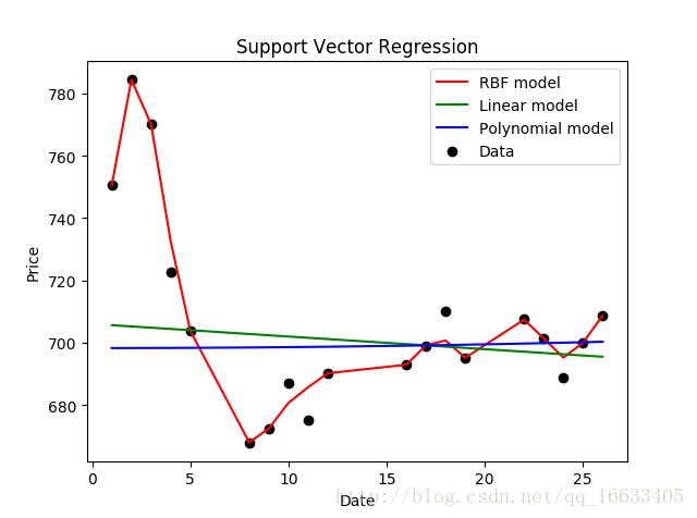
(1)kernel:核函数的类型,一般常用的有’rbf’,’linear’,’poly’,等如图4-1-2-1所示,发现使用rbf参数时函数模型的拟合效果最好。
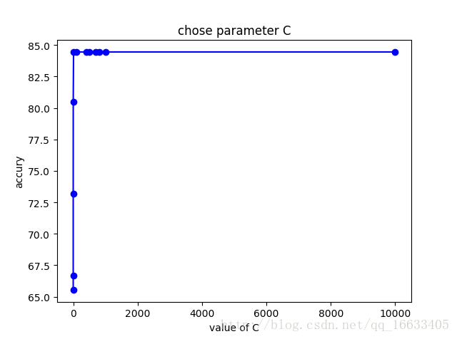
(2)C:惩罚因子。C表征你有多么重视离群点,C越大越重视,越不想丢掉它们。C值大时对误差分类的惩罚增大,C值小时对误差分类的惩罚减小。当C越大,趋近无穷的时候,表示不允许分类误差的存在,margin越小,容易过拟合;当C趋于0时,表示我们不再关注分类是否正确,只要求margin越大,容易欠拟合。如图4-1-2-2所示发现当使用1e3时最为适宜。
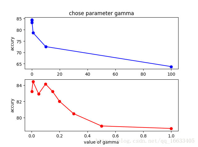
(3)gamma: 是’rbf’,’poly’和’sigmoid’的核系数且gamma的值必须大于0。随着gamma的增大,存在对于测试集分类效果差而对训练分类效果好的情况,并且容易泛化误差出现过拟合。如图4-1-2-3所示发现gamma=0.01时准确度最高。
可参考:https://blog.csdn.net/qq_16633405/article/details/70243030
四、源码:
import quandl
import numpy as np
from sklearn.linear_model import LinearRegression
from sklearn.svm import SVR
from sklearn.model_selection import train_test_split

#Get the stock data
# df = quandl.get("WIKI/AMZN")
# Take a look at the data
# print(df.head())

from jqdatasdk import *
auth('138xxxxxxx','a...4')
# quotes = pd.read_csv('002.csv')  # 读取训练数据

stock_code = '601318.XSHG'
start_date = '2016-02-05'
end_date = '2017-02-07'


df = get_price(stock_code, start_date, end_date, frequency='daily',skip_paused=False,fq='pre',fields=['open','high','low','close','money'])
print(df.head())

df = df[['close']]
print(df.head())


# A variable for predicting 'n' days out into the future
forecast_out = 30 #'n=30' days
#Create another column (the target or dependent variable) shifted 'n' units up
df['Prediction'] = df[['close']].shift(-forecast_out)
#print the new data set
print(df.tail())


### Create the independent data set (X)  #######
# Convert the dataframe to a numpy array
X = np.array(df.drop(['Prediction'],1))

#Remove the last 'n' rows
X = X[:-forecast_out]
# print(X)


### Create the dependent data set (y)  #####
# Convert the dataframe to a numpy array (All of the values including the NaN's)
y = np.array(df['Prediction'])
# Get all of the y values except the last 'n' rows
y = y[:-forecast_out]
# print(y)


# Split the data into 80% training and 20% testing
x_train, x_test, y_train, y_test = train_test_split(X, y, test_size=0.2)

# Create and train the Support Vector Machine (Regressor)
svr_rbf = SVR(kernel='rbf', C=1e3, gamma=0.1)
svr_rbf.fit(x_train, y_train)

# Testing Model: Score returns the coefficient of determination R^2 of the prediction.
# The best possible score is 1.0
svm_confidence = svr_rbf.score(x_test, y_test)
print("svm confidence: ", svm_confidence)


# Create and train the Linear Regression  Model
lr = LinearRegression()
# Train the model
lr.fit(x_train, y_train)

# Testing Model: Score returns the coefficient of determination R^2 of the prediction.
# The best possible score is 1.0
lr_confidence = lr.score(x_test, y_test)
print("lr confidence: ", lr_confidence)


# Set x_forecast equal to the last 30 rows of the original data set from Adj. Close column
x_forecast = np.array(df.drop(['Prediction'],1))[-forecast_out:]
# print(x_forecast)


# Print linear regression model predictions for the next 'n' days
lr_prediction = lr.predict(x_forecast)
print("linear regression model predictions for the next n days:\n",lr_prediction)
#将numpy数据存为csv
np.savetxt("lr_prediction.csv", lr_prediction, delimiter=',')

# Print support vector regressor model predictions for the next 'n' days
svm_prediction = svr_rbf.predict(x_forecast)
print("support vector regressor model predictions for the next n days:\n",svm_prediction)
#将numpy数据存为csv
np.savetxt("svm_prediction.csv", svm_prediction, delimiter=',')

#Original stock price
z = np.array(df['close'])
print("Original stock price for the next n days:\n",z[-forecast_out:])
np.savetxt("z.csv", z[-forecast_out:], delimiter=',')
五、执行结果
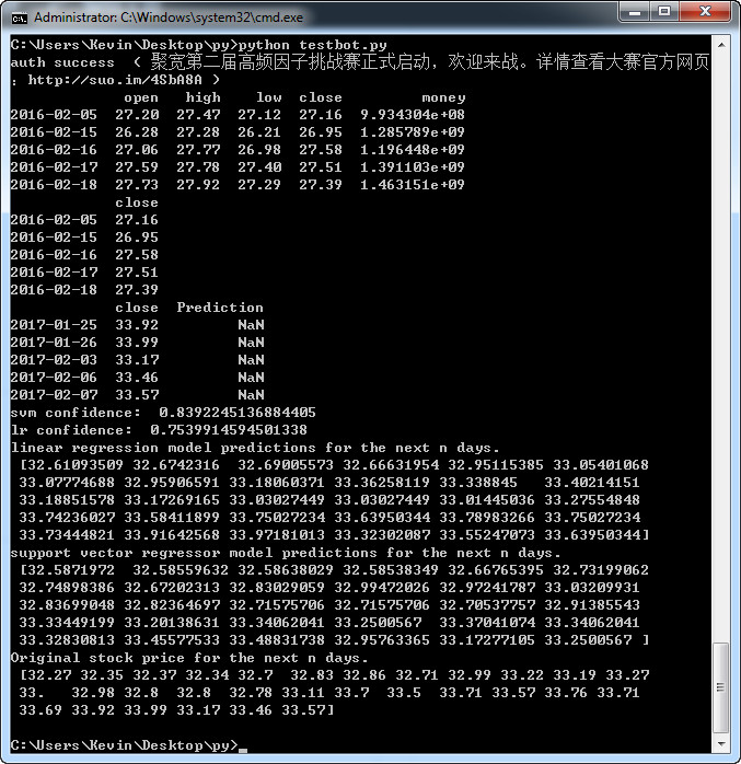
https://www.youtube.com/watch?v=EYnC4ACIt2g&t=9s
六、分析
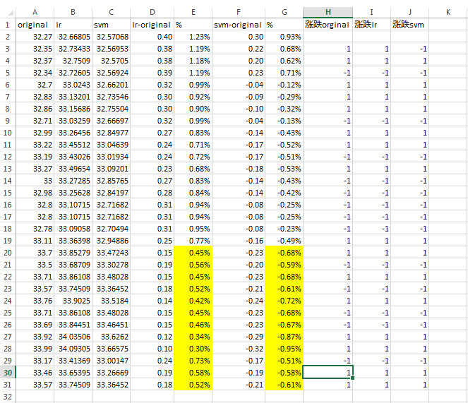
很明显,在执行“df['Prediction'] = df[['close']].shift(-forecast_out)”这句的时候,其实就是将未来30天的价格移到了现在,又去预测未来价格,使用了未来函数。
参考资料:
https://www.joinquant.com/view/community/detail/3f5f73ce173b157abac9aef8c0a71a96
https://www.youtube.com/watch?v=JgC9BEVS9Tk
https://www.youtube.com/watch?v=wxKLtaUryCw
https://www.youtube.com/watch?v=zwqwlR48ztQ